Getting Started

In order to get started with MPIFiles we first need some example datasets. These can be obtained by calling

download("https://media.tuhh.de/ibi/mdfv2/measurement_V2.mdf", "measurements.mdf")
download("https://media.tuhh.de/ibi/mdfv2/systemMatrix_V2.mdf", "systemMatrix.mdf")

which will download an MPI system matrix and an MPI measurement dataset into the current directory.

An MPI data file consists of a collection of parameters that can be divided into metadata and measurement data. We can open the downloaded MPI measurement data by calling

f = MPIFile("measurements.mdf")

f can be considered to be a handle to the file. The file will be automatically closed when f is garbage collected. The philosophy of MPIFiles.jl is that the content of the file is only loaded on demand. Hence, opening an MPI file is a cheap operation. This design allows it, to handle system matrices, which are larger than the main memory of the computer.

Using the file handle it is possible now to read out different metadata. For instance, we can determine the number of frames measured:

println( acqNumFrames(f) )
500

Or we can access the drive field strength

println( dfStrength(f) )
1×3×1 Array{Float64,3}:
[:, :, 1] =
 0.014  0.014  0.0

Now let us load some measurement data. This can be done by calling

u = getMeasurementsFD(f, frames=1:100, numAverages=100)

Then we can display the data using the PyPlot package

using PyPlot
figure(6, figsize=(6,4))
semilogy(abs.(u[1:400,1,1,1]))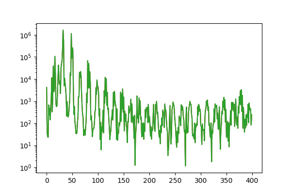

This shows a typical spectrum for a 2D Lissajous sampling pattern. The getMeasurementsFD is a high level interface for loading MPI data, which has several parameters that allow to customize the loading process. Details on loading measurement data are outlined in Measurements.

In the following we will first discuss the low level interface.